

Minimizing remote storage usage and synchronization time using deduplication and multichunking: Syncany as an example
Contents
Download as PDF: This article is a web version of my Master’s thesis. Feel free to download the original PDF version.
6. Experiments
The experiments in this thesis analyze and compare the different possible configurations based on the described algorithm and based on a set of carefully chosen datasets. The overall goal of all experiments is to find a good combination of configuration parameters for the use in Syncany — good being defined as a reasonable trade-off among the following goals:
- The temporal deduplication ratio is maximal
- The CPU usage is minimal
- The overall chunking duration is minimal
- The upload time and upload bandwidth consumption is minimal
- The download time and download bandwidth consumption is minimal
The scope of the experiments focuses on the three main phases of Syncany’s core. These phases strongly correlate to the architecture discussed in chapter 4.5. They consist of the chunking and indexing phase, the upload phase as well as the download and reconstruction phase (figure 6.1).
 |
| Figure 6.1: The experiments aim to optimize Syncany’s core phases in terms of deduplication ratio, processing time and bandwidth consumption. The main focus is on the chunking and indexing phase. |
Due to the high significance of the chunking and multichunking mechanisms, the biggest part of the experiment focuses on finding the optimal parameter configuration and on analyzing the interrelation between the parameters.
The following sections describe the surrounding conditions of the experiments as well as the underlying datasets.
6.1. Test Environment
Since Syncany runs on a client machine, all experiments were performed on normal user workstations.
The test machine for experiment 1 and 3 is a desktop computer with two 2.13 GHz Intel Core 2 Duo 6400 processors and 3 GB DIMM RAM (2x 1 GB, 2x 512 MB). It is located in the A5 building of the University of Mannheim, Germany. The machine is connected to the university network.
Since the setting for experiment 2 requires a standard home network connection, it is performed on a different machine. The test machine for this experiment is a Lenovo T400 notebook with two 2.66 GHz Intel Core 2 Duo T9550 processors and 4 GB DDR3 SDRAM. During the tests, the machine was located in Mannheim, Germany. The Internet connection is a 16 Mbit/s DSL, with a maximum upload speed of about 75 KB/s and a maximum download speed of 1.5 MB/s.
6.2. Parameter Configurations
The numerous possibilities to combine the parameters (as discussed in section 5.2) makes a complete analysis of all the combinations on all datasets unfeasable. As a consequence, the configurations chosen for this experiment are rather limited.
With the selection as indicated by the bold values in tables 5.1 and 5.2, there are in total 10 possible parameters. In particular, there are 12 chunkers, 4 multichunkers and 3 transformer chains, totalling to 144 different configurations. The following list is an excerpt of the configurations analyzed in this thesis. Appendix A shows the complete list:
- Custom-125-0/Fixed-4/Cipher
- Custom-125-0/TTTD-4-Adler32/Cipher
- Custom-125-0/TTTD-4-PLAIN/Cipher
- Custom-125-0/TTTD-4-Rabin/Cipher
- …
The syntax of the configuration string is as follows: Multichunker/Chunker/TransformationChain. Hyphens indicate the parameters of each of the components.
The syntax of the multichunker is represented by the type (always Custom), the minimum multichunk size (here: 125 KB or 250 KB), as well as the write pause (0 ms or 30 ms).
The chunker’s parameters include the type (Fixed or TTTD), the chunk size (4 KB — 16 KB) as well as the fingerprinting algorithm (only TTTD: Adler-32, PLAIN or Rabin).
The transformation chain’s parameters consist of a list of transformers (encryption and compression) in the order of their application. Possible values are Cipher (encryption), Gzip or Bzip2 (both compression).
6.3. Datasets
The datasets on which the experiments are conducted have been carefully chosen by the author based on the expected file types, file sizes, the amount of files to be stored as well as the expected change patterns to the files. To support the selection process, additional information has been collected from a small number of Syncany users and developers (35 participants). Appendix B shows details about what users were asked to do and what was analyzed. In particular, the pre-study collected the following data:
- Distribution of certain file types by size/count (e.g. JPG or AVI)
- Number/size of files that would be stored in a Syncany folder
Even though the results of this study are not representative of typical Syncany user data,1 they help by getting a better understanding of what data Syncany must expect. In particular, the data can be used to optimize the algorithms and/or the configuration parameters.
6.3.1. Pre-Study Results
This section briefly summarizes the results of the pre-study.
 |
 |
| Figure 6.2: Distribution of file types in the users’ Syncany folder by size | Figure 6.3: Distribution of file sizes in the users’ Syncany folder by size |
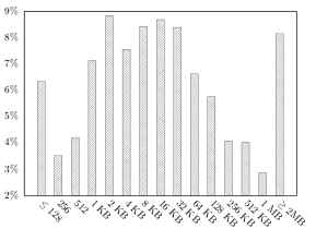
File sizes: The size distribution of the files in the users’ Syncany folders shows that over half of the files’ sizes range from 512 bytes to 32 KB. About 75% are smaller than 128 KB and only very few (8%) are greater than 2 MB (cf. figure 6.3).
Total size distribution: The total size of the users’ Syncany folders ranges from a few megabytes (minimum 9 MB) to over 600 GB for a single user. Most of the users store no more than 3.5 GB (67%), but also about 19% store more than 6 GB. The median share size is 1.5 GB.
Number of files: The amount of files varies greatly between the users. Some users only store a few dozen files, others have over 200,000 documents in their Syncany folders. About 51% store less than 3.400 files and about 75% less than 27,500 files. Only 10% store more than 100,000 files in the Syncany folders. The median number of files is 3,085.
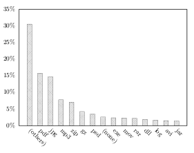
File types:2 There is a large variety of distinct file extensions in the users’ Syncany folders, many of which only occur very few times. Counting only those which occurred more than once (10 times), there are 2177 (909) distinct file extensions. If counted by file size, both PDF documents and JPG images each account for 15% of the users’ files. Another 30% consists of other file types (figure 6.2). When counting by the number of files, PDF files (JPG files) account for 10% (9%) of the users’ Syncany folders and office documents3 for about 8%.
6.3.2. Dataset Descriptions
Since the pre-study only captured a (non-representative) snapshot of the users’ potential Syncany folders, the datasets used for the experiments are only partially derived from its results. Instead, the actual datasets represent potential usage patterns and try to test many possible scenarios. In particular, they try to simulate the typical behavior of different user groups.
At time t0, each of the datasets consists of a certain set of files, the first version of the dataset. This version is then changed according to a change pattern — for instance by updating a certain file, adding new files or removing old files. Depending on the pattern, the dataset at time t can either differ by only very small changes or by rather big changes. Figure 6.4 illustrates a changing dataset over time. Each dataset version consists of a certain set of files. By altering one version of a dataset, a new version with new files is created.
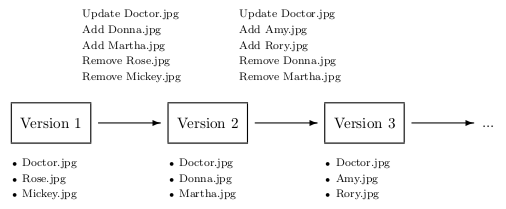 |
| Figure 6.4: Example of a dataset, updated by a user over time |
Consider a user working on an office document: If the document resides inside the monitored Syncany folder, it is very likely that changes to this document are rather small. If, however, the user only backs up the file in regular time intervals, changes are most likely bigger. Depending on the change pattern and file formats within a dataset, the deduplication algorithms are more or less effective. The following list briefly describes each of the datasets used for the experiments:
- Dataset A consists of a very small set of office documents which are gradually altered over time. Each dataset version at time t differs only by a single modification in one document. This dataset represents the usage pattern described above: A user works on a file and saves it regularly. Whenever the file is saved, the deduplication process is triggered by Syncany.
- Dataset B mostly contains file formats that are typically not modified by the user (such as JPG, PDF and MP3), but rather stay the same over time. With rare exceptions, subsequent dataset versions only differ by newly added files or by deleted files. This dataset represents a user group who mainly use Syncany to share files with others (or for backup).
- Dataset C contains a set of files that is composed of the 10 most frequent file types as found in the pre-study (by size). Each of the dataset versions differs by about 1–10 files from its predecessor. This dataset represents a daily-backup approach of a certain folder.
- Dataset D contains the Linux kernel sources in different versions — namely all released versions between 2.6.38.6 and 3.1.2. Each of the dataset versions represents one committed version within the version control system. This dataset is used to test how the algorithms perform on regularly changed plain text data. Using the source code of large open source projects is a common technique to test the efficiency of deduplication algorithms on plain text data [49,67].
| Dataset | Versions | Size | Files | Description | |
| A | Office documents | 50 | 5–9 MB | 24–25 | Collection of Microsoft Office and OpenOffice documents |
| B | Rarely modified | 50 | 400–900 MB | 700–1,900 | Collection of files that are rarely modified |
| C | Top 10 types | 50 | 100–150 MB | 230–290 | Collection of files based on the top 10 data types (by size) of the results of the pre-study |
| D | Linux kernels | 20 | 470–490 MB | 38,000–39,400 | Subsequent revisions of the Linux kernel source code |
Table 6.1: Underlying datasets used for the experiments.
Each of the experiments corresponds to one of Syncany’s core processes (as depicted in figure 6.1). The following sections describe each experiment and discuss their outcome.
6.4. Experiment 1: Chunking Efficiency
In order to reduce the overall amount of data, the efficiency of the chunking algorithm is the most important factor. The aim of this experiment is to find a parameter configuration that creates multichunks of minimal size, but at the same time does not stress the CPU too much.
The experiment compares the parameter configurations against each other by running the algorithms on the test datasets. It particularly compares runtime, processor usage, as well as the size of the resulting multichunks and index. This experiment helps analyzing the impact of each configuration parameter on the overall result of the algorithm. The goal is to find a configuration that matches the above aims (namely minimize result size, CPU usage and processing time).
The algorithm used for the experiment is very similar to the one described in chapter 5.3. In addition to the chunking and multichunking functionality, however, it includes code to create the index as well as mechanisms to calculate and measure the required parameters.
6.4.1. Experiment Setup
This experiment runs the Java application ChunkingTests on each of the datasets: It first initializes all parameter configurations, the chunk index, cache folders on the disk as well as an output CSV file. It then identifies the dataset versions of the given dataset (in this case represented by sub-folders) and finally begins the chunking and indexing process for each version.
The first version represents the initial folder status at the time t0. Each of the subsequent versions represent the folder status at time tn. In the first run (for t0), the index is empty and all files and chunks discovered by the deduplication algorithm are added. For subsequent runs, most of the discovered chunks are already present in the index (and hence in the repository) and do not need to be added.
For each version, the application records the index status and measures relevant variables. Most importantly, it records the size of the resulting multichunks, the CPU usage and the overall processing time using the current parameter configuration. Among others, each run records the following variables (for a detailed explanation of each variable see appendix C):
|
totalDurationSec totalChunkingDurationSec totalDatasetFileCount totalChunkCount totalDatasetSize totalNewChunkCount totalNewChunkSize totalNewFileCount totalNewFileSize totalDuplicateChunkCount |
totalDuplicateChunkSize totalDuplicateFileCount totalDuplicateFileSize totalMultiChunkCount totalMultiChunkSize totalIndexSize totalCpuUsage tempDedupRatio tempSpaceReducationRatio tempDedupRatioInclIndex |
tempSpaceRedRatioInclIndex recnstChunksNeedBytes recnstMultChnksNeedBytes recnstMultOverhDiffBytes recnst5NeedMultChnkBytes recnst5NeedChunksBytes recnst5OverheadBytes recnst10NeedMultChnkBytes recnst10NeedChunksBytes recnst10OverhBytes |
Figure 6.5: List of variables recorded by the ChunkingTests application for each dataset version.
Each dataset is analyzed 144 times (cf. section 6.2). For each parameter configuration, the application analyzes all the versions for the given dataset and records the results in a CSV file. For a dataset with 50 dataset versions, for instance, 7,200 records are stored.
6.4.2. Expectations
Both literature and the pre-testing suggest that a deduplication algorithm’s efficiency strongly depends on the amount of calculations performed on the underlying data as well as on how much data is processed in each step. The CPU usage and the overall processing time is expected to increase whenever a configuration parameter implies a more complex algorithm or each step processes a smaller amount of data. Each of the configuration parameters is expected to behave according to this assumption.
This is particularly relevant for the chunking algorithm, the fingerprinting algorithm and the compression mechanism. As indicated in chapter 3.4, coarse-grained chunking algorithms such as SIS with their rather simple calculations are most likely less CPU intensive than algorithms analyzing the underlying data in more detail. The two algorithms Fixed Offset (lower CPU usage) and Variable TTTD (higher CPU usage) used in these experiments are expected to behave accordingly. In terms of chunking efficiency, TTTD is expected to outperform the fixed offset algorithm due to its content-based approach.
The fingerprinting algorithms Adler-32, PLAIN and Rabin all perform significant calculations on the data. However, while PLAIN is mainly based on simple additions, it is expected to use fewer CPU than the other two. Since Rabin uses polynomials in its calculations, it will most likely use the most CPU out of the three. In terms of their efficiency, literature suggests that PLAIN is more effective than Rabin [38]. Since Adler-32 is not referenced in deduplication research, no statements can be made about its efficiency, speed or CPU usage. The three fingerprinting algorithms compete with the fixed offset algorithm which performs no calculations, but breaks files at fixed intervals. This method (in experiments called None) is expected to have the lowest average CPU usage, temporal deduplication ratio and total chunking duration (fastest).
In addition to the chunking and fingerprinting, Syncany’s algorithm compresses the resulting multichunks using Gzip or Bzip2. Naturally, using compression is much more CPU intensive than not using any compression at all (None). Hence, both processing time and CPU usage are expected to be very high compared to the compression-free method. However, the filesize of the resulting multichunks is most likely much smaller when using compression.
In terms of chunking efficiency, the chunk size parameter is expected to have the greatest impact. A small chunk size amplifies the deduplication effect and thereby decreases the resulting total multichunk size. On the contrary, it increases the number of necessary iterations and calculations which leads to a higher CPU usage.
In addition to the configuration parameters, the chunking efficiency is expected to greatly vary depending on the underlying dataset. Generally, the composition of file types within a dataset as well as the size of the dataset is expected to have a great influence on the overall deduplication ratio. Datasets with many compressed archive files, for instance, are expected to have a smaller deduplication ratio than datasets with files that change only partially when updated. Large datasets supposedly have a higher deduplication ratio than smaller ones, because the chances of duplicate chunks are higher with a growing amount of files.
Depending on how often files within a dataset are changed (change pattern), the temporal deduplication ratio is affected: Many changes on the same files most likely lead to a higher ratio (many identical chunks), whereas adding and deleting new files to the dataset is expected to have no or little influence on the ratio. Generally, the longer a dataset is used by a user, the higher the ratio is expected to be.
6.4.3. Results
The experiment compared 144 configurations on the four datasets described above (44 GB in total). Overall, the algorithms processed 6.2 TB of data and generated nearly 50 million chunks (totalling up to 407 GB of data). These chunks were combined to about 2.3 million multichunks (adding up to 330 GB of data). The total chunking duration of all algorithms and datasets sums up to 61 hours (without index lookups, etc.) and to a duration of over 10 days for the whole experiment.
The following sections present the results for both the best overall configuration as well as for each of the individual parameters. They look at how the parameters perform in terms of CPU usage, chunking duration as well as chunking efficiency.
6.4.3.1. Chunking Method
The chunking method generally decides how files are broken into pieces. A chunking algorithm can either emit fixed size chunks or variable size chunks.
The results of the experiment are very similar to what was expected before. Generally, the TTTD chunking algorithm provides better results in terms of chunking efficiency (temporal deduplication ratio) than the Fixed algorithm. However, it also uses more CPU and is significantly slower.
Over all test runs and datasets, the average temporal deduplication ratio of the TTTD algorithms is 12.1:1 (space reduction of 91.7%), whereas the mean for the fixed-size algorithms is 10.8:1 (space reduction of 90.7%). Looking at the total multichunk sizes, the average space savings using TTTD are about 4.6% when comparing them to the fixed-size algorithms, i.e. the multichunks generated by TTTD are generally smaller than the ones by the fixed-size algorithms.
 |
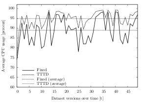 |
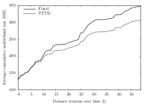
| Figure 6.6: Average cumulative multichunk size over time, compared by chunking algorithm (dataset A) | Figure 6.7: Average CPU usage over time, compared by the chunking algorithm (dataset C) |
For dataset C, the space savings of the variable-size algorithms are a lot higher than the average. The multichunks created with a TTTD algorithm are about 13.2% smaller than the ones using fixed-size algorithms. That equals to space saving of about 810 KB per run. Figure 6.6 illustrates this difference over time: Both TTTD and the fixed-size algorithms create about 130 MB of multichunks in the first run. However, the variable-size chunking algorithms save space with each dataset version in tn — totalling up to a difference of over 40 MB after 50 versions (306 MB for TTTD and 347 MB for the fixed-size algorithms).
In terms of CPU usage, the fixed-size algorithms use less processing time than the variable-size algorithms. On average, TTTD algorithms have a 3.6% higher CPU usage percentage (average of 93.7%) than the fixed-size ones (average of 90.0%). In fact, the TTTD CPU percentage is above the fixed-size percentage in almost every run. Figure 6.7 shows the average CPU usage while chunking dataset D using both fixed-size and variable-size algorithms. With a value of 94.8%, the TTTD average CPU usage is about 6% higher than the fixed-size average (88.8%).
Similar to the CPU usage, the less complex fixed-size chunking method performs better in terms of speed. However, while the CPU usage only slightly differs between the two chunking methods, the chunking duration diverges significantly. On average, the fixed-size algorithms are more than 2.5 times faster than variable-size algorithms. Over all datasets and runs, the average chunking duration per run for the fixed-size algorithms is about 4.1 seconds, whereas the average duration for the TTTD algorithms is 10.7 seconds. Depending on the underlying dataset, this effect can be even stronger: For dataset B, the fixed-size algorithms are on average 14.3 seconds faster than the TTTD algorithms, which is almost three times as fast (average per-run chunking duration of 7.8 seconds for fixed-size and 22.2 seconds for TTTD). After 50 runs, this time overhead adds up to almost 12 minutes (6.5 minutes for fixed-size, 18.5 minutes for TTTD).
6.4.3.2. Fingerprinting Algorithm
The fingerprinting algorithm is responsible for finding natural break points as part of a content-based chunking algorithm (here: only TTTD). The better the algorithm performs, the higher the number of duplicate chunks (and the lower the total file size of the new chunks).
 |
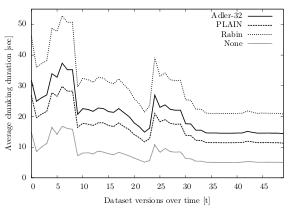 |
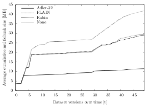
| Figure 6.8: Average cumulative multichunk size over time, compared by fingerprinting algorithm (dataset A) | Figure 6.9: Average chunking duration, clustered by fingerprinting algorithm (dataset B) |
The results of the experiment show that the Adler-32 fingerprinter outperforms the other algorithms in terms of chunking efficiency in all datasets. Over all test runs, the Adler-32 average temporal deduplication ratio is 14.7:1 (space reduction of 93.2%) — compared to a ratio of only 11.2:1 for the PLAIN algorithm (space reduction of 91.1%). With a ratio of 10.3:1 (space reduction of 90.3%), the Rabin algorithm performs the worst out of all four. In fact, its average temporal deduplication ratio is worse than the average of the fixed-size chunking algorithms (ratio of 10.8:1, space reduction of 90.7%).
Figure 6.8 illustrates the different chunking efficiency of the fingerprinting algorithms for dataset A. In the first run, all algorithms create multichunks of similar size (about 3.6 MB). After the data has been changed 50 times, however, the multichunks created by Adler-32 add up to only 11.4 MB, whereas the ones created by Rabin are almost four times as big (41.8 MB). Even though the multichunks created by PLAIN and the fixed-size algorithm are significantly smaller (about 29 MB), they are still 2.5 times bigger than the ones created using the Adler-32 fingerprinter.
For dataset C, Adler-32 creates about 25% smaller multichunks than the other algorithms: After 50 test runs, the average size of the multichunks created from dataset C is 245.5 MB (temporal deduplication ratio of 24.4:1, space reduction of 95.9%), whereas the output created by the other fingerprinters is larger than 325 MB. Compared to PLAIN, for instance, Adler-32 saves 80.6 MB of disk space. Compared to Rabin, it even saves 102.5 MB.
Looking at dataset B, the space savings are not as high as with the other datasets: The temporal deduplication ratio is 19.4:1 (space reduction of 94.8%) and the multichunk output is 1,462 MB — compared to 1,548 MB for PLAIN (deduplication ratio of 18.4:1, space reduction of 94.5%). Even though the space reduction after 50 dataset versions is not as high compared to the other datasets, it still saves 85.9 MB.
The CPU usage of the fingerprinters largely behaves as expected. With an average of 93.5%, Rabin has a higher average CPU usage than PLAIN with 92.4% and much higher than the fixed-size algorithms with 90%. Surprisingly, Adler-32 uses the most processor time (average CPU usage of 95.1%) — even though its algorithm is solely based on additions and shift-operations (as opposed to calculations based on irreducible polynomials in the Rabin fingerprinting algorithm).
In terms of chunking duration, the fixed-size algorithms are certainly faster than the variable-size algorithms based on TTTD (as shown in section 3.4.3.1). In fact, they take about half the time than the PLAIN algorithms and less than a third than the algorithms using the Rabin fingerprinter. Over all datasets and test runs, the average chunking duration for algorithms with fixed-offset chunking is 4.1 seconds, for PLAIN based algorithms it is 8.3 seconds, for Adler-32 based algorithms it is 10.0 seconds and for Rabin based algorithms it is 13.7 seconds.
Figure 6.9 shows the differences in the chunking duration over time for dataset B: Algorithms using Rabin as fingerprinting mechanism are significantly slower than algorithms using other or no fingerprinters. Rabin is on average about 9 seconds slower than PLAIN and Adler-32 and over 20 seconds behind the algorithms without fingerprinter (fixed). Totalling this extra time over 50 changesets, Adler-32 is about 7.5 minutes faster than Rabin, PLAIN about 11 minutes and fixed-size algorithms over 18 minutes.
6.4.3.3. Compression Algorithm
After a multichunk has been closed (because the target size is reached), it is further compressed using a compression algorithm. When analyzing the chunking efficiency in regard to what compression algorithm has been used, the results in all datasets show that Bzip2 produces the smallest multichunks, but at the same time has a higher CPU usage than the other options Gzip and None. While these results are consistent throughout all datasets, the difference between the compression algorithms is marginal.
Over all datasets and test runs, the Bzip2 algorithm creates an output that is about 2% smaller than the one created using Gzip and about 42% smaller than without the use of a compression algorithm. The average temporal deduplication ratio with Bzip2 is 13.06:1 (space reduction of 92.3%), whereas when using Gzip, the ratio is 12.6:1 (space reduction of 92.0%). Without any compression, the average temporal deduplication ratio is 9.6:1 (space reduction of 89.6%).
 |
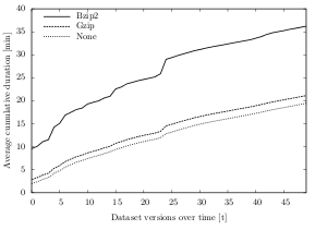 |
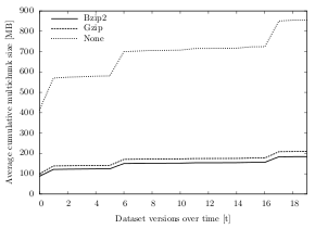
| Figure 6.10: Average cumulative multichunk size over time, clustered by compression algorithm (dataset D) | Figure 6.11: Average cumulative overall duration over time, clustered by compression algorithm (dataset B) |
For datasets A, B and C, the temporal deduplication ratio of Bzip2 and Gzip after 50 changes differs by only 0.3, i.e. the size of the generated multichunks is almost identical (max. 2% spread). Expressed in bytes, the Gzip/Bzip2 spread is only about 100 KB for dataset A (27.8 MB and 27.7 MB), 8 MB for dataset B (1,492 MB and 1,500 MB) and 6 MB for dataset C (300 MB and 294 MB).
For dataset D, the difference of the multichunk sizes between Gzip and Bzip2 is slightly higher (13% spread, about 24 MB), but very small compared to the spread between compression (Gzip/Bzip2) and no compression. Figure 6.10 illustrates these differences for dataset D over time: Starting in the first run, the algorithms with Gzip or Bzip2 compression create multichunks of under 100 MB, whereas the multichunks created by the algorithms without compression are about four times the size (412 MB). Over time, this 312 MB spread grows even bigger and the cumulative multichunk size of Gzip and Bzip2 add up to about 200 MB, compared to 855 MB for the no compression algorithms (655 MB spread).
In terms of CPU usage, the algorithms with Bzip2 use an average of 94%, while the ones using the Gzip algorithm use an average of 92.4%. Without compression, the CPU usage average over all datasets and test runs is 91.9%. While Bzip2 consumes the most processing time on average, the percentage is not constantly greater than the CPU usage numbers of Gzip and no compression. In fact, in dataset A and B, the algorithms without compression and the Gzip algorithms use more CPU than the Bzip2 algorithms.
Regarding the speed of the compression algorithms, Bzip2 is significantly slower than the other two compression options. With regard to all datasets and test runs, Bzip2 has an average overall per-run duration4 of 20.6 seconds, Gzip has a moderate speed (average 12.5 seconds) and not compressing the multichunks is the fastest method (11.5 seconds). Gzip is about 63% faster than Bzip2, not compressing is about 78% faster. The difference between Gzip and not compressing the multichunks is only about 8%.
Looking at dataset B in figure 6.11, for instance, the average cumulative overall duration using Bzip2 is much higher than for the options Gzip and None. In the first run, the algorithms using Gzip run less than 3 minutes, the ones without any compression only 2 minutes. The ones using Bzip2 as compression algorithm, however, run more than three times longer (9.5 minutes). This significant speed difference carries on throughout all test runs and leads to an overhead of about 15 minutes between Bzip2 and Gzip and about 17 minutes between Bzip2 and the no compression algorithms.
6.4.3.4. Chunk Size
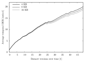
The chunk size parameter defines the target size of the resulting chunks of the algorithm. Generally, smaller chunk sizes lead to a higher deduplication ratio, but require more CPU time.
Even though these statements match the results of the experiments, the impact of the parameter is not as high as expected. In fact, independent of the chosen chunk size (4 KB, 8 KB or 16 KB), the algorithm produces very similar results. Chunking efficiency, CPU usage and total chunking duration only differ marginally in their results.
 |
 |
| Figure 6.12: Average temporal deduplication ratio over time, clustered by chunk size (dataset C) | Figure 6.13: Average chunking duration over time, clustered by the chunk size (dataset B) |
Over all datasets and test runs, the maximum temporal deduplication ratio for a chunk size of 4 KB is 26.7:1 (space reduction of 96.2%). For 8 KB, the best temporal deduplication ratio is 25.8:1 (space reduction of 96.1%) and for 16 KB it is 25.1:1 (space reduction of 96.0%).
Figure 6.12 shows the temporal deduplication ratio for dataset B. Independent of the chunk size, the average ratio develops almost identically for the three parameter values. After 50 snapshots of the dataset, the ratios are 20.1:1 (4 KB chunks), 19.3:1 (8 KB chunks) and 18.7:1 (16 KB chunks). Expressed in absolute values, the total cumulated multichunk size is 305.6 MB using 4 KB chunks, 316.7 MB using 8 KB chunks and 328.1 MB using 16 KB chunks. The results for other datasets have even closer ratios. The deduplication ratios of dataset B only differ by 0.16 (18.7:1 for 4 KB chunks, 18.6:1 for 8 KB chunks and 18.5:1 for 16 KB chunks) and of dataset A by only 0.10.
The average CPU usage, clustered by the three parameters, is very similar. With 4 KB chunks, the average CPU usage over all test runs is 95.1%, for 8 KB chunk size it is 94.9% and for 16 KB chunk size it is 95.5%. In fact, for datasets B and C, the mean deviation of the CPU usage per test run is only 0.5% and 0.4%, respectively. Only dataset A shows significant differences in the CPU usage: Its average deviation is 7.7%, its median deviation 4.7%.
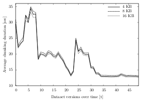
Similar to the CPU usage, the chunking duration is also hardly affected by the size of the created chunks. Independent of the parameter value, the overall chunking duration is very similar. As table 6.2 shows, the average chunking duration per test run and dataset are completely decoupled from the chunk size. Even for dataset B, for which the cumulated chunking duration is over 15 minutes, the time difference after the last run is less than one minute. For the smaller datasets A and C, the average duration is almost identical (for A about 10 seconds, for C about 3 minutes, 38 seconds).
| Max. Deduplication Ratio | Avg. Chunking Duration | |||||
| Chunk Size | Dataset A | Dataset B | Dataset C | Dataset A | Dataset B | Dataset C |
| 4 KB | 26.33:1 | 20.17:1 | 26.76:1 | 10 sec | 15:29 min | 3:38 min |
| 8 KB | 25.68:1 | 20.00:1 | 25.81:1 | 10 sec | 15:52 min | 3:38 min |
| 16 KB | 24.47:1 | 19.77:1 | 25.15:1 | 9 sec | 15:11 min | 3:37 min |
Table 6.2: Maximum temporal deduplication ratio per dataset (left) and average chunking duration per dataset (right), both clustered by chunk size.
Figure 6.13 illustrates the average chunking durations for dataset B, clustered by the chunk size: The more files are changed/updated/new in between the indexing runs, the longer it takes to complete the chunking process. However, while the duration differs significantly in each run (about 35 seconds in the sixth run vs. about 12 seconds for the last run), it only marginally varies for the different chunk sizes (average deviation of 0.5 seconds).
6.4.3.5. Write Pause
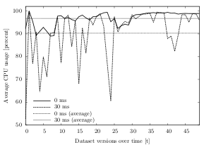
The write pause parameter defines the number of milliseconds the chunking algorithm sleeps after each multichunk. The parameter is meant to artificially slow down the chunking time in order to lower the average CPU usage.
The results of the experiments show that the algorithms without a sleep time (0 ms) have an 11% higher average CPU usage — compared to the ones with a 30 ms write pause in between the multichunks. On average, the 0 ms-algorithms use 98.8% CPU, whereas the 30 ms-algorithms use 87.8%.
Figure 6.14 shows the effects of the write pause parameter during the chunking and indexing process of dataset B. Without sleep time, all of the values are above 89% and the average CPU usage is 96.7% — i.e. the CPU is always stressed. With a short write pause in between the multichunks, the average is reduced to 90.3%.
 |
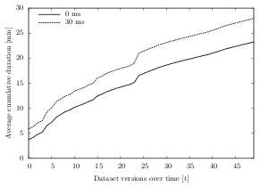 |
| Figure 6.14: Average CPU usage over time, clustered by the write pause (dataset B). | Figure 6.15: Cumulative chunking duration over time, clustered by write pause (dataset B). |
While the parameter has a positive effect on the CPU usage, it lengthens the overall chunking duration. On average, 30 ms-algorithms run 19.8% longer than the ones without pause. For the datasets in the experiments, this longer duration ranges from a few seconds for small datasets (additional 6 seconds for dataset A) to many minutes for larger ones (additional 5 minutes for dataset B). Broken down to the chunking process of a single snapshot, the additional time is rather small: 0.12 seconds for dataset A, 5.6 seconds for dataset B and 1.3 seconds for dataset C.
Figure 6.15 illustrates the cumulative duration5 while chunking dataset B. Since the underlying calculations and algorithms are identical, the two curves develop similarly — only with a vertical shift. In fact, the correlation of both curves is 0.99.
The write pause parameter has no impact on the chunking efficiency, i.e. on the temporal deduplication ratio, because it does not alter the algorithm itself, but rather slows it down.
6.4.3.6. Multichunk Size
The multichunk size parameter controls the minimum size of the resulting multichunks. Rather than influencing the chunking efficiency, it aims at maximizing the upload bandwidth and minimizing the upload duration (see experiment 2 in section 6.5). Even though the impact of the parameter on the chunking efficiency is small, it must be part of the analysis.
The results of the experiments show that the average DER with a minimum multichunk size of 250 KB is slightly higher than when 125 KB multichunks are created. Over all datasets and test runs, the average temporal deduplication ratio is 11.8:1 (space reduction of 91.5%) for algorithms with 250 KB multichunk containers and 11.7:1 (space reduction of 91.4%) for algorithms with 125 KB multichunks. The difference in the deduplication ratio is below 0.1 for datasets A, B and C, but as high as 0.6 for dataset D.
In terms of CPU usage, algorithms using 125 KB multichunks use less CPU, because they have about double the amount of write pauses in the chunking process. 125 KB algorithms use an average of 91.7% CPU, whereas algorithms creating 250 KB multichunks use 93.9% CPU.
The additional write pauses in the 125 KB algorithms also affect the overall duration. On average, algorithms creating 250 KB chunks are about 8% faster than algorithms creating 125 KB chunks. The overall average duration per run for the 125 KB option is 15.4 seconds, whereas the overall average for the 250 KB option is 14.3 seconds.
Looking at dataset C, for instance, the mean difference in the initial run is only about 9 seconds (53 seconds for 250 KB algorithms, 62 seconds for 125 KB algorithms). Over time, i.e. after chunking and indexing 50 versions, the average cumulated difference is still only 21 seconds (363 seconds for 125 KB algorithms, 342 seconds for 250 KB algorithms).
6.4.3.7. Overall Configuration
Having analyzed the individual parameters and their behavior in the experiment, this section focuses on the overall configuration of these parameters. In order to finally choose a suitable configuration for Syncany, this section is of particular importance. While the previous sections focused on only one parameter at a time, this section is able to weigh the parameters against each other and make statements about individual parameters in the overall context.
Deduplication ratio: Table 6.3 gives an excerpt of the best overall parameter configuration with respect to the average deduplication ratio (full table in appendix D). The results of the experiment confirm the expectations to a large extent on all of the four datasets.
| Rank | Algorithm Configuration | A | B | C | D | Average | |
| 1 | Custom-250-*/TTTD-4-Adler32/Bzip2-Cipher | 15.35 | 12.88 | 15.43 | 32.67 | 16.68 | |
| 2 | Custom-125-*/TTTD-4-Adler32/Bzip2-Cipher | 15.33 | 12.84 | 15.40 | 30.92 | 16.45 | |
| 3 | Custom-250-*/TTTD-8-Adler32/Bzip2-Cipher | 15.13 | 12.80 | 15.00 | 30.56 | 16.22 | |
| 4 | Custom-250-*/TTTD-4-Adler32/Gzip-Cipher | 15.37 | 12.82 | 15.37 | 28.31 | 16.14 | |
| 5 | Custom-125-*/TTTD-4-Adler32/Gzip-Cipher | 15.39 | 12.82 | 15.38 | 27.99 | 16.11 | |
| 6 | Custom-125-*/TTTD-8-Adler32/Bzip2-Cipher | 15.12 | 12.75 | 14.96 | 29.00 | 16.01 | |
| 7 | Custom-250-*/TTTD-16-Adler32/Bzip2-Cipher | 14.55 | 12.67 | 14.68 | 28.74 | 15.71 | |
| 8 | Custom-250-*/TTTD-8-Adler32/Gzip-Cipher | 15.16 | 12.73 | 14.94 | 26.37 | 15.70 | |
| 9 | Custom-125-*/TTTD-8-Adler32/Gzip-Cipher | 15.17 | 12.73 | 14.94 | 26.11 | 15.67 | |
| 10 | Custom-125-*/TTTD-16-Adler32/Bzip2-Cipher | 14.53 | 12.63 | 14.66 | 27.29 | 15.51 | |
| … | … | … | … | … | … | … | |
| 67 | Custom-250-*/TTTD-16-Rabin/Cipher | 6.00 | 11.23 | 9.31 | 5.53 | 8.46 | |
| 68 | Custom-125-*/TTTD-16-Rabin/Cipher | 6.00 | 11.23 | 9.31 | 5.53 | 8.46 | |
| 69 | Custom-250-*/TTTD-8-Rabin/Cipher | 5.26 | 11.24 | 9.81 | 5.67 | 8.40 | |
| 70 | Custom-125-*/TTTD-8-Rabin/Cipher | 5.26 | 11.24 | 9.81 | 5.67 | 8.40 | |
| 71 | Custom-250-*/TTTD-4-Rabin/Cipher | 3.99 | 11.27 | 9.74 | 5.79 | 8.03 | |
| 72 | Custom-125-*/TTTD-4-Rabin/Cipher | 3.98 | 11.27 | 9.74 | 5.79 | 8.03 |
Table 6.3: Average temporal deduplication ratio over all datasets (as ratio:1), clustered by algorithm configuration and sorted by the average. The full list can be found in appendix D.
With regard to the deduplication ratio and the derived space reduction percentage, the chunking method and the fingerprinting algorithm have the strongest influence on the result: In terms of the chunking method, the variable-size algorithm TTTD is used in all of the top third algorithm configurations (first 24). However, it is also used in 18 of the worst 24 algorithms.6
Looking at the fingerprinters, the Adler-32 algorithm has proven most effective for all of the analyzed datasets. In the overall ranking, 16 out of 18 Adler-32 algorithms appear in the first third of the table and all of them are present in the first half. The other fingerprinters are distributed over the whole ranking, with PLAIN mostly in the mid-range and Rabin performing worst. In fact, none of the top 24 algorithms use the Rabin fingerprinter and only two of the first half do.
Besides chunker and fingerprinter, the compression algorithm is of particular relevance in terms of deduplication ratio: Over 80% of the best 24 algorithms use compression — equally divided between Gzip and Bzip2 (10 configurations each). Most of the algorithms without compression (18 of 24) reside at the end of the table, with the lowest average temporal deduplication ratio.
Even though the chunk size was expected to have a high influence on the chunking efficiency, the impact is small compared to the other parameters. For the chunk sizes 4 KB and 8 KB, about 83% of the algorithm configurations are in the top third of the list (41.6% each) and about 17% are algorithms with 16 KB chunks. Particularly the two options 4 KB and 8 KB have a similar distribution in the list and do not seem to differ much with regard to the deduplication ratio. The 16 KB option, however, differs in its impact on the DER: About 70% of the algorithms in the bottom half of the list use 16 KB chunks.
The multichunk size is by far the parameter with the least relevance to the deduplication ratio: 125 KB and 250 KB algorithm configurations are equally distributed amongst the ranking. 19 of the 36 algorithms with 250 KB multichunks are in the upper half of the list, 17 in the bottom half. Conversely, 17 of 36 algorithms with 125 KB chunks are in the top half of the table, 19 in the bottom half. In fact, the difference is so marginal that the 125 KB and 250 KB configurations with otherwise identical parameters are often very close together in the list (if not right behind each other).
Looking at the absolute ratios in table 6.3, the difference among the configurations is quite big: While the best algorithm configuration Custom-250-*/TTTD-4-Adler32/Bzip2-Cipher has an average deduplication ratio of 16.7:1 (space reduction of 94%), the worst configuration Custom-125-*/TTTD-4-Rabin/Cipher only reaches an average of 8:1 (space reduction of 87.5%).
When looking at the differences between the datasets, the deduplication ratio differs significantly: The ratio reaches an average of 32.6:1 (space reduction of 96.9%) in dataset D for the best configuration and less than half for dataset C (ratio of 12.9:1, space reduction of 92.2%). For the worst configuration, the best average ratio is reached by dataset B with 11.3:1 (space reduction of 92.1%) and the worst ratio by dataset A (ratio of 4:1, space reduction of 74.8%). Depending on the data in the dataset, the spread between the best and the worst configuration can be higher or lower. While the best/worst-spread in dataset B is only 1.6 (12.9:1 and 11.3:1), the ratio difference for dataset D is 26.9 (32.7:1 and 5.8:1).
Total duration: The overall duration behaves almost reverse to the temporal deduplication ratio. Many well-performing parameters in terms of chunking efficiency slow down the overall chunking process. Table 6.4 gives an excerpt of the ranking with regard to the overall per-run duration (full table in appendix E).
| Rank | Algorithm Configuration | A | B | C | D | Average |
| 1 | Custom-250-0/Fixed-8/Cipher | 0.10 | 9.09 | 1.70 | 12.92 | 4.72 |
| 2 | Custom-250-0/Fixed-16/Cipher | 0.10 | 8.60 | 1.64 | 14.58 | 4.75 |
| 3 | Custom-125-0/Fixed-16/Cipher | 0.09 | 10.62 | 1.64 | 15.16 | 5.42 |
| 4 | Custom-250-0/Fixed-4/Cipher | 0.10 | 10.88 | 1.88 | 16.82 | 5.76 |
| 5 | Custom-250-0/Fixed-16/Gzip-Cipher | 0.14 | 11.14 | 2.22 | 15.56 | 5.80 |
| 6 | Custom-125-0/Fixed-8/Cipher | 0.10 | 11.99 | 1.71 | 15.13 | 5.84 |
| 7 | Custom-125-0/Fixed-4/Cipher | 0.10 | 10.84 | 1.96 | 17.72 | 5.88 |
| 8 | Custom-125-0/Fixed-16/Gzip-Cipher | 0.14 | 11.00 | 2.20 | 16.91 | 5.91 |
| 9 | Custom-250-0/Fixed-8/Gzip-Cipher | 0.14 | 11.66 | 2.28 | 15.89 | 6.01 |
| 10 | Custom-125-0/Fixed-8/Gzip-Cipher | 0.14 | 11.52 | 2.28 | 17.41 | 6.15 |
| … | … | … | … | … | … | … |
| 139 | Custom-250-30/TTTD-16-Rabin/Bzip2-Cipher | 0.90 | 54.34 | 13.69 | 46.29 | 25.72 |
| 140 | Custom-250-30/TTTD-8-Rabin/Bzip2-Cipher | 1.02 | 54.32 | 13.31 | 47.99 | 25.84 |
| 141 | Custom-250-30/TTTD-4-Rabin/Bzip2-Cipher | 1.13 | 56.06 | 13.27 | 48.94 | 26.48 |
| 142 | Custom-125-30/TTTD-16-Rabin/Bzip2-Cipher | 0.99 | 57.88 | 14.60 | 53.20 | 27.87 |
| 143 | Custom-125-30/TTTD-8-Rabin/Bzip2-Cipher | 1.11 | 58.72 | 14.24 | 54.79 | 28.23 |
| 144 | Custom-125-30/TTTD-4-Rabin/Bzip2-Cipher | 1.26 | 60.13 | 14.27 | 56.16 | 28.86 |
Table 6.4: Average overall per-run duration over all datasets in seconds, clustered by algorithm configuration and sorted by the average. The full list can be found in appendix E.
As it is visible from the table, the factor with the gratest influence on the overall speed of the algorithm is the chunking method: While TTTD produces the better DER results, the fixed-size chunking algorithms are significantly faster. Overall, all of the 17 top algorithm configurations use a fixed-size chunker instead of a variable-size chunker. About 66% of the fixed-size configurations are in the top third of the ranking and over 72% in the first half. Conversely, less than 23% of the TTTD-based algorithms are in the list of the best 48 configurations.
With the values of this experiment, the second most important factor is the write pause: The top 12 of all algorithm configurations have no write pause in between the multichunks, i.e. the write pause parameter is set to 0 ms. Overall, about 66% of the algorithms in the first third have no write pause. On the contrary, 30 of the 48 last configurations have the parameter set to 30 ms.
Apart from the chunking method, compression is the parameter with the second highest impact: Depending on the compression method, algorithms can be signficantly slower. For this ranking, 77% of the algorithms without compression can be found in the first half of the list. The Bzip2 algorithm in particular is not used in any of the first 48 configurations and in only two of the first 72 algorithms. In fact, the last 19 configurations use the Bzip2 algorithm to compress their multichunks. Compared to that, Gzip is much more prominent in the top part of the list: About 44% of the upper half algorithms use the Gzip compression.
When TTTD is used, the fingerprinting method is an important factor to influence the speed. In the experiments, the Rabin method has proven to be by far the slowest: In the first third of all configurations, none of the algorithms used Rabin as fingerprinter and only two of the first half did. Conversely, about 94% of all algorithms using Rabin can be found in the bottom half of the list — 12 of them on the ranks 133–144. Compared to that, the other fingerprinters do not have that much influence on the speed. PLAIN occurs in 15 of the first 48 algorithms, Adler-32 in only 9.
The last two parameters, multichunk size and chunk size, have no visible impact on the overall duration at all. The algorithm configurations with the multichunk sizes 125 KB and 250 KB distribute evenly in the ranking: 45% of 125 KB algorithms in the top half, 54% in the bottom half — and vice versa for the 250 KB algorithms. For the chunk sizes 4 KB, 8 KB and 16 KB, the situation is similar. For all of them, there are around 33% of each configuration in the first third/half.
CPU usage: The average processor usage is in many properties similar to the overall duration. As with the duration, some DER-improving parameters increase the CPU percentage. Table 6.5 shows an excerpt of the best algorithm configurations with regard to the CPU usage. Since the amount of data in dataset A was very small and a test run was often faster than a second, the CPU measurements are not reliable. Average values and ranking do not include the measurements of dataset A.
| Rank | Algorithm Configuration | A | B | C | D | Average |
| 1 | Custom-125-30/Fixed-16/Cipher | 67.12 | 78.58 | 65.28 | 54.30 | 66.05 |
| 2 | Custom-125-30/Fixed-8/Cipher | 75.44 | 80.86 | 66.14 | 53.55 | 66.85 |
| 3 | Custom-125-30/Fixed-16/Gzip-Cipher | 70.36 | 81.92 | 70.02 | 52.50 | 68.15 |
| 4 | Custom-125-30/Fixed-4/Cipher | 72.28 | 82.70 | 67.84 | 57.45 | 69.33 |
| 5 | Custom-125-30/Fixed-8/Gzip-Cipher | 79.82 | 83.26 | 70.56 | 55.60 | 69.81 |
| 6 | Custom-125-30/Fixed-4/Gzip-Cipher | 76.42 | 84.04 | 71.88 | 56.85 | 70.92 |
| 7 | Custom-250-30/Fixed-8/Cipher | 85.22 | 85.72 | 76.60 | 54.15 | 72.16 |
| 8 | Custom-250-30/Fixed-16/Cipher | 70.88 | 84.02 | 76.20 | 58.20 | 72.81 |
| 9 | Custom-250-30/Fixed-4/Cipher | 78.50 | 87.50 | 77.90 | 58.90 | 74.77 |
| 10 | Custom-250-30/Fixed-16/Gzip-Cipher | 74.96 | 86.92 | 80.18 | 59.05 | 75.38 |
| … | … | … | … | … | … | … |
| 139 | Custom-125-0/TTTD-16-Rabin/Gzip-Cipher | 105.90 | 99.02 | 99.34 | 85.60 | 94.65 |
| 140 | Custom-125-0/TTTD-8-Rabin/Gzip-Cipher | 103.82 | 99.52 | 99.40 | 85.05 | 94.66 |
| 141 | Custom-250-0/TTTD-16-Rabin/Gzip-Cipher | 103.80 | 99.08 | 99.24 | 86.05 | 94.79 |
| 142 | Custom-250-0/TTTD-8-Rabin/Cipher | 106.78 | 99.04 | 99.14 | 87.15 | 95.11 |
| 143 | Custom-250-0/TTTD-4-Rabin/Cipher | 111.20 | 97.98 | 99.40 | 88.35 | 95.24 |
| 144 | Custom-250-0/TTTD-8-Rabin/Gzip-Cipher | 103.24 | 99.60 | 99.22 | 87.70 | 95.51 |
Table 6.5: Average CPU usage in percent, clustered by algorithm configuration and sorted by the average. Due to unreliable measurements in dataset A, its values are ignored in ranking and average. The full list can be found in appendix F.
The greatest influence on the average CPU usage is the write pause parameter: Most of the algorithm configurations with the lowest average CPU usage have set the parameter to 30 ms. Out of the 48 top configurations in the ranking, 44 are 30 ms-configurations. Conversely, only 4 of the 0 ms-configurations are in the top third and only 14 in the top half.
The parameter with the second greatest impact on the processor usage is the chunking method: The top 13 algorithms in the ranking use a fixed-size chunker and nearly 90% of all fixed-size algorithms can be found in the top half of the ranking.
Apart from the chunking method and the write pause, the fingerprinting method has a great impact as well. In particular, algorithms using the Rabin fingerprinting method have a rather high CPU usage compared to other fingerprinters. In fact, 21 of the 36 algorithms using Rabin can be found in the bottom third of the list — 12 of them even on the last positions.
The impact of the multichunk size is not insignificant: 30 out of the 72 algorithms with 125 KB multichunks are in the top third of the ranking, whereas only 18 of the 250 KB algorithms appear in the table. That is about 63% of the first third are algorithms creating 125 KB multichunks.
The other parameters, namely chunk size and compression, are only marginally relevant in the overall context: In terms of compression, not compressing has slight advantages for the overall configuration. About 58% of the non-compressing algorithms are in the top half of the ranking, whereas over 53% of the algorithms using compression are in the bottom half. The chunk size has even less impact on the overall configuration. All algorithms with 4 KB, 8 KB and 16 KB chunks are equally distributed in the ranking, with about 33% of each in the first third/half.
| Lowest CPU | Lowest Duration | Highest DER | |
| Chunking Algorithm | Fixed | Fixed | TTTD |
| Fingerprinting Algorithm | None | None | Adler-32 |
| Compression Algorithm | None | None | Bzip2 |
| Chunk Size | & 16 KB | 16 KB | 4 KB |
| Write Pause | 30 ms | 0 ms | indiff. |
| Multichunk Size | 125 KB | 250 KB | 250 KB |
Table 6.6: Best configuration parameters with regard to the respective aims of minimizing the CPU usage, minimizing the total duration as well as maximizing the temporal deduplication ratio.
Table 6.6 illustrates the best values with regard to the respective goals that have been derived from the results of the experiments.
6.4.4. Discussion
After analyzing the results of the experiments, this section aims at interpreting and discussing these results in the scope of Syncany. In particular, its goal is to find a suitable overall algorithm configuration — with regard to Syncany’s environment and requirements.
In the typical Syncany use case, the application runs in the background and the user is not supposed to be disturbed by it (low CPU usage). In some cases, the user’s goal is to simply backup some data (duration marginally relevant). In other cases, it is to share files with other users as quickly as possible (duration very relevant). Similarly, sometimes the remote storage is paid per GB, in other cases the storage is limited in size (high DER desired).
The experiment above targeted these goals and tried to optimize the generic deduplication algorithm by changing the input parameters. As the results show, many of the parameters perform quite well in one or two of these goals, but not in all of them. In fact, many of the DER-improving parameters such as Adler-32 or Bzip2 perform badly in terms of overall duration or CPU usage. Vice versa, parameters with better speed and CPU performance such as the fixed-size chunking method perform worse in terms of space savings.
With regard to the goal of Syncany as an end-user application, one of the most basic requirements is to make its usage easy and non-disruptive to other applications. It must hence be the first priority to reduce the CPU usage and hide the deduplication process from end-users. Chunking efficiency and overall duration must be considered secondary — at least for this case.7
Taking the reduction of CPU usage as the primary goal, all of the algorithm configurations analyzed in the experiment show a rather weak performance: Most of the configurations with a relatively high average deduplication ratio have CPU averages around 90%. For a background end-user application, this value is unacceptable. Instead, a much lower average should be targeted in the selection of a suitable algorithm. Values around 20–30% are acceptable, given that the application only needs resources for a limited time.
While the results of the experiments help identifying parameters with extremely bad CPU impact, they do not clearly state a winner in terms of overall configuration. Even the best configurations have far higher averages than desired. In fact, the high CPU usage indicates that other means are necessary to limit processor usage.
The write pause parameter, for instance, is intended to fulfill this exact purpose, but has not succeeded to reliably control processor usage limits: While the parameter can lower the average CPU usage, it does not allow setting a maximum percentage or take the differences of the underlying data into account. Due to the many small text files in dataset D, for instance, the average processor usage is much lower than in dataset C. Using the same algorithm, the resulting difference in the CPU usage is often over 20%.
Instead of having a single fixed write pause parameter such as 30 ms, an effective algorithm should dynamically adjust this parameter depending on the measured CPU usage. An algorithm could, for instance, increase the write pause up to 100 ms or 150 ms, if the CPU is stressed and lower it when the percentage is below the maximum.
Having the other goals in mind, some of the other parameters must be tolerated as-is despite their bad CPU performance. Variable-size chunking methods and some of the corresponding fingerprinting algorithms, for instance, have a rather high impact on the temporal deduplication ratio. Even though their average processor usage is high in the experiments, a dynamic write pause parameter could artificially slow down the algorithm to decrease the processor usage. In fact, since all configurations can be slowed down, it makes sense to only eliminate the parameter values that evidently cause a significantly higher CPU usage.
The most noticeable parameter is the Rabin fingerprinting algorithm: As already discussed in section 6.4.3.2 (and also visible in tables 6.5 and F.1), algorithms using Rabin and Adler-32 have a higher average CPU usage than other algorithms. However, while Adler-32 has a superior average deduplication ratio and overall runtime, Rabin performs quite bad in all measures — and is hence not suitable as potential parameter.
The second parameter with obvious negative influence on the average CPU usage is the compression algorithm Bzip2. Compared to Gzip, it uses more CPU cycles and appears in many of the worst performing algorithm configurations. Additionally, it performs exceptionally bad in terms of overall duration. In particular when combining Bzip2 with a potentially higher (or dynamic) write pause parameter, the algorithm would run slower by the orders of magnitude. It, too, is not suitable as a potential parameter for Syncany.
Assuming that the write pause parameter can counteract the potentially bad CPU impact of the other parameters, the second most important factor is the efficiency of the chunking algorithm: Given that remote storage often costs money, minimizing the data to store also reduces the total cost of storage. Additionally, reducing the overall amount of data also reduces the time to upload/download it from the storage and thereby accelerates the overall time of synchronization between two Syncany clients.
As already discovered in section 6.4.3.7, the parameter with the greatest positive influence on the deduplication ratio is the Adler-32 fingerprinting algorithm. It performs well for all datasets and has — despite the relatively high processor usage — no negative properties. In fact, compared to the other fingerprinters, the achieved space savings due to Adler-32 are remarkably high and cannot compare to the other fingerprinting mechanisms.
Given the outstanding performance of the algorithm, it makes sense to choose Adler-32 as the fingerprinter of choice for Syncany. And since that implies a variable-size chunker, TTTD is by definition the most suitable chunking method. Conversely, that disqualifies the fixed-size chunker and the PLAIN fingerprinter as primary choice for Syncany’s deduplication algorithm.
| Chosen Value | Explanation | |
| Chunker | TTTD | Variable-sized chunking allows for higher space savings than fixed-size chunking. |
| Fingerprinter | Adler-32 | Adler-32 outperforms the other options in terms of deduplication. Rabin performs bad in all measures. |
| Compression | Gzip | Bzip2 is too slow and the no compression option performs bad on pure text files. |
| Chunk Size | 4 KB | The chunk size is almost indifferent in regard to all measures. 4 KB chunks deliver better deduplication results. |
| Write Pause | ≥ 30 ms | The 30 ms option reduces CPU usage, but not enough for Syncany. Dynamic write pauses are desirable. |
| Multichunk Size | 250 KB | The analyzed values are largely indifferent. The 250 KB variant has a higher DER. |
Table 6.7: Chosen values for Syncany based on the results of experiment 1.
From the perspective of the deduplication ratio, the last parameter with significant impact on the space savings is the no compression parameter. While Bzip2 is already disqualified due to high CPU usage and extremely long overall runtime, both Gzip and no compression are still viable options. However, while Gzip performs acceptable with regard to reducing the size of the resulting multichunks, not using compression has shown to be very ineffective. As shown in section 6.4.3.3, it performs bad on all datasets, but in particular on plain text files (dataset D). For Syncany, this fact eliminates no compression as a viable option.
The two left over parameters chunk size and multichunk size have hardly any impact on any of the measures. All parameter values share similar CPU usage percentages, average duration values and average temporal deduplication ratios. With regard to these findings, the best parameter for Syncany in the respective category is the one with the highest DER — even though its difference to the other values is small. For the chunk size, the best value in that regard is 4 KB (as opposed to 8 KB and 16 KB). For the multichunk size parameter, this value is 250 KB.
Table 6.7 shows the values chosen for Syncany and summarizes the reasoning behind the decision. In the syntax of this thesis, the chosen overall algorithm configuration for Syncany is Custom-250-30/TTTD-4-Adler32/Gzip-Cipher.
In the rankings (as described in section 6.4.3.7), this algorithm ranks at 4 of 72 in the DER ranking (appendix D), at 64 of 144 in the duration ranking (appendix E) and at 62 of 144 in the CPU ranking (appendix F).
While the deduplication ranking is undoubtably very good, the other two only place the algorithm at the end of the top half. Even though that seems bad, it must be examined with care. Most of the top algorithms in the duration ranking are 0 ms-algorithms and/or Fixed-algorithms. After eliminating these options, it ranks in the top third. Similarly, the rank in the CPU table is only partially relevant, given that the CPU usage can be regulated with a higher (or dynamic) write pause parameter.
Overall, the chosen algorithm is a good trade-off between space reduction, CPU usage and runtime.
6.5. Experiment 2: Upload Bandwidth
Experiment 1 measured the chunking efficiency and tried to minimize the total size of the created chunks and multichunks. The goal of the experiment was to reduce the data that has to be transferred to the remote storage. While chunking efficiency is an important factor to reduce the upload bandwidth consumption, it is not the only relevant determinant. As discussed in chapter 5.1.3, the number of required upload requests can have a large impact on the request overhead and the upload duration.
The goal of this experiment is to prove that the multichunk concept maximizes the overall upload bandwidth independent of the storage type. In particular, it aims at reducing the overall upload duration (and thereby maximize the total upload bandwidth). It furthermore analyzes the upload behavior with regard to different types of storage.
The experiment is based on the results of the previous experiment and measures the upload duration and upload bandwidth with regard to the chosen chunk size and storage type.
6.5.1. Experiment Setup
The experiment runs the Java application UploadTests using the results from experiment 1: As input, it takes the average chunk sizes for each test run and dataset (for the target chunk sizes 4 KB, 8 KB and 16 KB and the multichunk sizes 125 KB and 250 KB) as well as the total size of the created multichunks per run (data to upload each run).
Using these average chunk sizes, it creates dummy chunks (random data) and uploads these chunks as files to the remote storage (FTP, S3 and IMAP). It measures the upload time and then derives the upload bandwidth. In order to cancel out interferences and factor in request latencies, it uploads each chunk multiple times and only stores the average duration.
For each dataset version, the application records the bytes uploaded, the upload duration and the derived upload bandwidth in KB/s. It furthermore derives the total upload duration as if the whole multichunk data were to be uploaded (linearly scaled).
6.5.2. Expectations
The multichunk concept aims at reducing the latency produced by uploading too many small files to a remote storage. By grouping chunks into multichunks, the number of upload requests is reduced. This reduction is expected to lower the total request overhead from the individual upload requests, reduce latency and increase the total upload bandwidth. Independent of the type of remote storage storage, the size of the uploaded payload is expected to directly influence the upload speed.
In particular, using smaller chunk sizes (4 KB, 8 KB and 16 KB) is expected to result in a significantly lower upload bandwidth than using larger chunk sizes (125 KB and 250 KB). That is using small chunks, the total upload time is expected to be higher than if multichunks are used.
Furthermore, it is expected that the type of storage has a direct influence on the average absolute upload speed, but not on the relative speed amongst the different chunk sizes. IMAP, for instance is expected to have a significantly lower average upload bandwidth than FTP or S3, because the payload is encoded using Base64. It is, however, not expected to behave differently than other storage types with respect to the chunk size.
6.5.3. Results
The experiment uploaded 514.1 MB to three different types of storage (FTP, S3 and IMAP). Overall, 20,910 chunks of different sizes were uploaded in the total duration of almost four hours.
The following sections present the results of the upload experiment. The analysis first looks at the size of the uploaded chunks in order to verify the multichunk concept and then identifies differences in the upload times between different storage types.
6.5.3.1. Chunk Size
The upload bandwidth is measured by dividing the number of uploaded bytes by the upload duration. In Syncany, a higher bandwidth is desirable, because it minimizes the time it takes to upload chunks and metadata. It thereby minimizes the time for clients to synchronize changes to the repository.
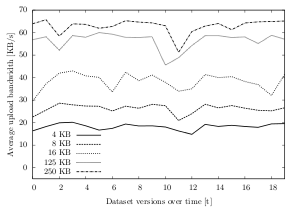
The results of this experiment show that the upload bandwidth largely behaves as expected: Over all datasets and storage types, the average upload bandwidth using 4 KB chunks is only about 21.2 KB/s, whereas the bandwidth using 250 KB chunks is about 60.5 KB/s. The upload speed of using the other chunk sizes lies in between those values: Using 8 KB chunks, the speed is about 31.1 KB/s, using 16 KB chunks, the speed is about 41.3 KB/s and using 125 KB chunks, the speed is about 57.0 KB/s.
Looking at dataset D in figure 6.16, for instance, the upload bandwidth spread can be observed over time: While the speed stays near 55 KB/s when using 125 KB chunks and around 65 KB/s for 250 KB chunks, the bandwidth never reaches 30 KB/s when 8 KB chunks are used and not even 20 KB/s when 4 KB chunks are used.
 |
 |
| Figure 6.16: Average upload bandwidth over time, clustered by chunk size (dataset D). | Figure 6.17: Cumulative average upload duration over time, clustered by chunk size (dataset C). |
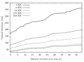
Since the upload bandwidth is derived from the upload duration, its value behaves accordingly. On average, using 250 KB chunks is 4.4 times faster than using 4 KB chunks, about 2.8 times faster than using 8 KB chunks and about 1.8 times faster than using 16 KB chunks. The upload duration difference between 250 KB and 125 KB chunks is marginal: Using 250 KB chunks is about 13% faster than using 125 KB chunks. When excluding IMAP, this difference is even lower (7%).
Figure 6.17 shows these results for dataset C over time. With an initial upload duration of about 168 minutes using 4 KB chunks, compared to only 34 minutes when using 250 KB chunks, the 4 KB option is almost five times slower (134 minutes). This spread grows over time to a difference of over 4.5 hours (84 minutes using 250 KB chunks, 361 minutes using 4 KB chunks). While the spread from the 250 KB option to the 8 KB and 16 KB options is not as large as to the 4 KB option, it is significantly larger than between the 125 KB and 250 KB: Even after 50 uploads, the average cumulated 125/250 KB difference is less than 9 minutes, whereas the 16/250 KB spread is about 54 minutes.
6.5.3.2. Storage Type
The remote storage is the location at which the chunks or multichunks are stored. Depending on the underlying application layer protocol, chunks are transferred differently and the average upload bandwidth differs.
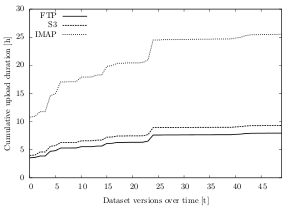
The results of the experiment show that the average upload bandwidth strongly depends on the storage type: Out of the three protocols within this experiment, the one with the highest average upload bandwidth is FTP with 54.1 KB/s, followed by the REST-based Amazon S3 with 49.1 KB/s and the e-mail mailbox protocol IMAP with only 23.6 KB/s (cf. figure 6.19).
 |
 |
| Figure 6.18: Average cumulative upload duration over time, clustered by storage type (dataset B). | Figure 6.19: Average upload bandwidths, clustered by dataset and storage type (all datasets). |
While the bandwidth differs in its absolute values, the relative difference between the protocol speeds is very similar: FTP, for instance, is around 10% faster than Amazon S3 (± 2% in each dataset) and about 2.3 times faster than IMAP (± 3% in each dataset).
Figure 6.18 illustrates these different upload durations for dataset B: While the initial upload using FTP takes on average 3.5 hours and less than four hours using Amazon S3, storing the same amount of data in an IMAP mailbox takes over 10 hours. Over time, the spread grows to about 81 minutes between FTP and S3 (7.9 hours for FTP, 9.3 hours for S3) and to over 17 hours between FTP and IMAP (25.5 hours for IMAP).
6.5.4. Discussion
Having seen the results of the experiment, the multichunk concept has proven very effective to maximize the overall upload bandwidth. Independent of the underlying storage type, combining smaller chunks reduces the upload time and eliminates wait times. Due to a reduction of upload requests, the protocol-dependent latencies are minimized. For instance, instead of having 100 upload requests using 4 KB chunks, two requests with 250 KB multichunks are sufficient. The experiment has shown that the concept works regardless of the storage and independent of the dataset.
For Syncany, this method is valuable in two ways. First, it reduces the overall synchronization time between two or more Syncany clients. By increasing the upload speed, clients can publish their file changes faster and thereby enable a faster exchange of metadata and chunks. Second, it mitigates the effects of the different storage types. While the concept is not able to converge the speed of all protocols to the client’s maximum upload speed, it shifts the focus from the protocol-dependent request overhead to the speed of the actual upload connection.
Especially when looking at Syncany’s minimal storage interface (as described in chapter 4.5.4), decoupling from the specifics of the storage protocols reduces more of the protocol’s peculiarities. With protocols as different as Amazon S3 and IMAP, increasing the chunk size adds an extra layer of abstraction to this interface. Instead of having to deal with heavy-weight request headers or a high number of small requests in each Syncany plug-in, they behave alike even if the protocol differs significantly.
The overall algorithm configuration in experiment 1 includes 250 KB multichunks (as opposed to 125 KB multichunks). In experiment 1, the primary goal was the reduction of the total disk space, whereas the goal of experiment 2 was reducing upload bandwidth. The results for both goals show that 250 KB multichunks are the best option.
However, while the multichunk concept improves the upload speed, it can lead to an overhead in the download and reconstruction process. Experiment 3 analyzes this behavior in more depth.
6.6. Experiment 3: Multichunk Reconstruction Overhead
In typical deduplication systems, reconstruction only depends on the retrieval of the necessary chunks. In Syncany’s case, however, chunks are stored in multichunks. While this reduces the total number of required upload/download requests, it can potentially have negative effects on the total reconstruction time and bandwidth. Instead of having to download only the required chunks, Syncany must download the corresponding multichunks.
This experiment calculates the download overhead (multichunk reconstruction overhead) caused by the multichunk concept. It particularly illustrates the difference of the overhead when the last five (ten) dataset versions are missing and shows how the total overhead behaves when no version is present on the client machine.
6.6.1. Experiment Setup
The experiment has two parts: The first part is conducted as part of the ChunkingTests application in experiment 1:8 After each test run on a dataset version, the multichunk overhead is calculated based on the current and previous states of the chunk index. This part of the experiment does not actually perform measurements on algorithms or transfer any data. Instead, the results are calculated from the intermediate output of experiment 1.
In particular, the overhead is calculated as follows: For each file in the current dataset version Vn and each chunk these files are assembled from, a lookup is performed on the index of version Vn-5 (last five versions missing), Vn-10 (last ten versions missing) or V∅ (initial state, no chunks/multichunks). If the chunk is present in this dataset version, it does not need to be downloaded, because it already exists locally. If the chunk is not present, the corresponding multichunk needs to be downloaded.
In the latter case, both chunk and multichunk are added to a need-to-download list. Once each file has been checked, the total sizes of the chunks and the total sizes of the multichunks are added up. The quotient of the two is the multichunk reconstruction overhead (in percent). Alternatively, the absolute overhead (in bytes) can be expressed as difference between the two sums.
 |
(6.1) |
The measure expresses how many additional bytes have to be downloaded to reconstruct a certain dataset version because multichunks are used. It compares the amount that would have been downloaded without the use of multichunks to the amount that actually has to be downloaded. The value of the overhead is influenced by the time of last synchronization (last locally available dataset version), the size of the multichunks and the changes of the underlying data.
The second part of the experiment runs the Java application DownloadTests. This application is very similar to the UploadTests application from experiment 2. Instead of measuring the upload speed, however, it measures the download speed of the different storage types in relation to the chunk and multichunk size. As the UploadTests application, it takes the average chunk sizes from experiment 1 as input and uploads chunks with the respective size to the remote storage. It then downloads the chunk multiple times and measures the download bandwidth (including the latency). Using the average download speeds from this application, the total download time per dataset version can be calculated.
6.6.2. Expectations
The multichunk concept reduces the amount of upload requests. Instead of uploading each chunk separately, they are combined in a multichunk container. The bigger these multichunks are, the fewer upload requests need to be issued. Since fewer upload requests imply fewer request overhead, the overall upload time is reduced (see section 6.5 for details).
While this concept helps reducing the upload time, it is expected to have negative effects on the download time. Since chunks are stored in multichunk containers, the retrieval of a single chunk can mean having to download the entire multichunk. Due to the fact that the reconstruction overhead strongly depends on the size of the multichunks, this effect is expected become worse with a larger multichunk size. Looking at the multichunk sizes chosen for this experiment (cf. table 5.1), the 250 KB multichunks are expected to produce higher traffic than the 125 KB multichunks.
Besides the multichunk size, another important factor is time: The reconstruction overhead is expected to increase over time when many of the remote updates are missed. In the initial indexing process at time t0, all chunks inside all multichunks are used. When a client attempts to download the current dataset version V0, the overhead is zero (or even negative due to multichunk compression). Over time, some of the chunks inside the multichunks are only useful if older versions are to be restored. If a client attempts to download version Vn without having downloaded any (or a few) of the other versions before, many of the multichunks may contain chunks that are not needed for this dataset version.
The results of the experiment are expected to reflect this behavior by showing a higher overhead when the last ten dataset versions are missing (compared to when only five versions are missing). The highest overhead is expected when version Vn is reconstructed without having downloaded any previous versions (full reconstruction). The download time is expected to behave accordingly.
6.6.3. Results
The results of this experiment largely confirm the expectations. Both time and multichunk size affect the reconstruction overhead. While the size of the multichunk has a rather small effect, the changes made over time impact the results significantly. In addition to these two dimensions, the impact of the underlying dataset is larger than anticipated.
6.6.3.1. Multichunk Size
When reconstructing a file, a client has to download a certain amount of multichunks to retrieve all the required chunks. The greater the multichunk size, the greater is the chance that unnecessary chunks have to be downloaded. As expected, the results show that 250 KB multichunks cause a higher download volume than 125 KB multichunks.
Table 6.8 illustrates the average multichunk reconstruction overhead over all datasets and test runs. Using 250 KB multichunks, the overhead is 15.2%, whereas the average using 125 KB multichunks is about 13.0% (full reconstruction). The difference is similar when the last five (ten) dataset versions are missing: Using 250 KB multichunks, the average overhead is about 9.0% (10.4%), using 125 KB multichunk, the average overhead is about 6.1% (7.9%).
| Overhead, all missing | Overhead, 10 missing | Overhead, 5 missing | ||||
| 125 KB | 250 KB | 125 KB | 250 KB | 125 KB | 250 KB | |
| Dataset A | 10.8% | 11.4% | 8.4% | 12.0% | 9.3% | 12.6% |
| Dataset B | 2.5% | 4.8% | 0.8% | 1.7% | 0.9% | 2.1% |
| Dataset C | 7.8% | 14.8% | 3.1% | 7.7% | 2.5% | 7.0% |
| Dataset D | 57.7% | 52.1% | 36.5% | 34.9% | 20.2% | 22.9% |
| 13.0% | 15.2% | 7.9% | 10.4% | 6.1% | 9.0% | |
Table 6.8: Average multichunk overhead for a full reconstruction and when the last five/ten versions are missing, clustered by the multichunk size.
Broken down to datasets, the overhead percentages are very different: While the average full multichunk reconstruction overhead for dataset B is only 4.8% (250 KB multichunks) and 2.5% (125 KB multichunks), the average for dataset D is about 52.1% (250 KB multichunks) and 57.7% (125 KB multichunks). Expressed in MB, using 250 KB (125 KB) multichunks requires an additional download of about 22 MB (11 MB) for dataset B (dataset size ±600 MB, ±1,000 files) and an additional 219 MB (243 MB) for dataset D (dataset size ±400 MB, ±36,000 files). When the last five dataset versions are missing, the average overhead caused by the multichunk concept are 2.1 MB (250 KB multichunks) and 1.1 MB (125 KB multichunks) for dataset B and 55 MB (250 KB multichunks) and 61 MB (125 KB multichunks) for dataset D. When the last ten versions are missing, the average overhead is 3.6 MB (250 KB multichunks) and 1.9 MB (125 KB multichunks) for dataset B and 119 MB (250 KB multichunks) and 133 MB (125 KB multichunks) for dataset D.
Figure 6.20 and 6.21 illustrate the absolute multichunk reconstruction size for dataset C over time. Figure 6.20 compares the total size of the version to the full reconstruction size using 125 KB multichunks and 250 KB multichunks. Figure 6.21 compares the impact of the multichunk size on the reconstruction size when the last five (ten) versions are missing.
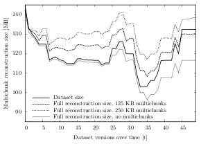 |
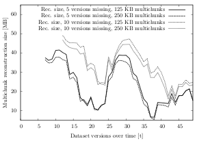 |
| Figure 6.20: Full reconstruction size over time, clustered by multichunk size (dataset C). | Figure 6.21: Reconstruction size over time, clustered by missing versions and multichunk size (dataset C). |
Independent of the multichunk size, the full reconstruction size for dataset C is almost always larger than the actual size of the dataset. Compared to that, reconstructing the dataset version without the use of multichunks always requires downloading fewer data. Figure 6.20 shows that full reconstruction with 125 KB multichunks requires downloading an average of 124 MB for the dataset version, whereas reconstruction with 250 KB multichunks requires on average of 130 MB (difference of only 5%). When reconstructing the version by downloading the individual chunks, the average download volume is 115 MB, which is less than the average size of the dataset version (119 MB).
After an initial full download of a dataset, updating to the latest version requires downloading fewer multichunks. Figure 6.21 shows how many multichunks need to be downloaded to bring the existing version to the latest state. In particular, it shows that the download size grows when more versions are missing in between the local version and the newest version. For dataset C, the average reconstruction size if five versions are missing is 23.7 MB when 125 KB multichunks are used, compared to 22.2 MB when 250 KB multichunks are used. If ten versions are missing, the average reconstruction size for 125 KB multichunks is 34.5 MB and for 250 KB multichunks it is 32.4 MB.
6.6.3.2. Changes over Time
With regard to the multichunk concept, the factor time is of particular importance. Especially when looking at how files are added, changed and removed from a dataset, the differences in the reconstruction behavior are huge. The previous section briefly showed that the reconstruction size depends on the multichunk size. In addition to the multichunk size, the amount and type of changes over time is also relevant.
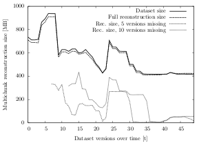 |
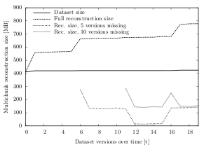 |
| Figure 6.22: Reconstruction size over time, clustered by the number of missing versions (dataset B). | Figure 6.23: Reconstruction size over time, clustered by the number of missing versions (dataset D). |
Looking at dataset B in figure 6.22, for instance, the reconstruction size is significantly lower if there already is a local version present. Over time, when files are altered in the dataset, some of the remote multichunks become partially irrelevant for the reconstruction, while others do not. These partially irrelevant multichunks have to be downloaded completely in order to get the necessary chunks. The more often a dataset is changed, the higher is the amount of data an unsynchronized client has to download for reconstruction. For dataset B, the average reconstruction size is 115 MB if the last five versions are missing and 179 MB if the last ten are missing. Compared to that, the average full reconstruction size is 557 MB, with an average dataset size of 569 MB. If more versions were in between the local and the current version, the average amount would be even higher.
While the full reconstruction size in dataset B is almost always below the respective size of the dataset version, reconstructing dataset D requires a significant overhead. Figure 6.23 shows the multichunk reconstruction size over time for dataset D. With the exception of the initial run, the full reconstruction size is always much higher than the dataset size. After only one additional version, reconstructing version V1 requires downloading 557 MB (overhead of 137 MB to the dataset size, +32.6%). After 19 other versions, this overhead grows to almost double the size of the dataset: For a 424 MB dataset, the client needs to download 778 MB of multichunks (overhead of 354 MB, +83.4%). On average, the full reconstruction size for dataset D is 647 MB.
While the full reconstruction size behaves differently for dataset B and D, it behaves similar when the last five or ten versions are missing: On average, a client needs to download 111 MB to update its local version if five versions are missing and 174 MB if ten are missing.
6.6.3.3. Download Bandwidth
Even though the multichunk concept implies a higher download volume, the bandwidths measured using the DownloadTests application show that the total download time is still shorter when multichunks are used. In particular, the experiments proof that independent of the storage type, using 250 KB multichunks is the best option with regard to the download time.
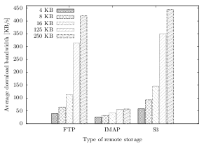 |
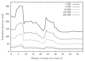 |
| Figure 6.24: Average download bandwidth, clustered by chunk/multichunk size and storage type (all datasets). | Figure 6.25: Average download duration over time, clustered by chunk/multichunk size (dataset B). |
On average, the download speed behaves similar to the upload speed (as measured in experiment 2). Independent of the storage type, the download bandwidth is much higher if multichunks are used (figure 6.24). For FTP (Amazon S3), the average download bandwidth is 39 KB/s (58 KB/s) using 4 KB chunks, compared to 421 KB/s (444 KB/s) using 250 KB multichunks. Similar to the upload speed, the IMAP download bandwidth is much lower than that: Using 4 KB chunks, IMAP only reaches 25 KB/s and only 57 KB/s if 250 KB multichunks are used. The bandwidths of the other chunk/multichunk sizes lie in between those values.
In combination with the reconstruction size per version, the download bandwidths can be used to calculate the total download duration (table 6.9). For the chunk sizes 4 KB, 8 KB and 16 KB, the value of Need-to-Download Chunks was used for the calculation. For the multichunk sizes 125 KB and 250 KB, the value of Need-to-Download Multichunks was used as a basis (cf. equation 6.1).
Table 6.9 shows the results of the estimated download time for each dataset. On average, using 250 KB multichunks is almost three times faster than using 4 KB chunks. When IMAP is excluded from the calculation, the spread in download duration is even higher: Downloading the necessary 4 KB chunks takes about seven times longer than downloading the required 250 KB multichunks.
| Using Chunks | Using Multichunks | ||||||
| 4 KB | 8 KB | 16 KB | 125 KB | 250 KB | |||
| Set A | FTP | 110 sec | 68 sec | 39 sec | 16 sec | 12 sec | |
| IMAP | 172 sec | 138 sec | 109 sec | 89 sec | 86 sec | ||
| Amazon S3 | 75 sec | 48 sec | 30 sec | 14 sec | 11 sec | ||
| Set B | FTP | 224 min | 139 min | 80 min | 29 min | 22 min | |
| IMAP | 350 min | 282 min | 221 min | 168 min | 164 min | ||
| Amazon S3 | 153 min | 97 min | 62 min | 26 min | 21 min | ||
| Set C | FTP | 47 min | 29 min | 17 min | 7 min | 5 min | |
| IMAP | 74 min | 60 min | 48 min | 38 min | 38 min | ||
| Amazon S3 | 32 min | 21 min | 13 min | 6 min | 5 min | ||
| Set D | FTP | 177 min | 108 min | 62 min | 35 min | 25 min | |
| IMAP | 277 min | 219 min | 171 min | 201 min | 187 min | ||
| Amazon S3 | 121 min | 76 min | 48 min | 32 min | 24 min | ||
Table 6.9: Calculated average dataset download times, clustered by chunk/multichunk size, dataset and storage type.
Looking at dataset D, for instance, the average download time using FTP and 4 KB chunks is about 176 minutes (almost 3 hours) for 420 MB of chunks. Compared to that, downloading the necessary 250 KB multichunks for reconstruction only takes 25 minutes — even though almost 640 MB multichunks need to be downloaded. Similarly, reconstructing a version in dataset B using Amazon S3 and 4 KB chunks takes about 153 minutes (2.5 hours; 530 MB chunk data), while downloading the 560 MB multichunk data only takes 21 minutes (250 KB multichunks).
Figure 6.25 shows these different download times for dataset B over time for an FTP storage: For each of the versions in dataset B, downloading the necessary chunks/multichunks takes only about 25–50 minutes if 125/250 KB multichunks are used, but always over two hours if the data is stored in 4 KB chunks. On average, downloading the necessary chunk data takes about 3.7 hours if 4 KB chunks are used and about 22 minutes if the repository stores 250 KB chunks.
6.6.4. Discussion
Experiments 1 and 2 have shown that the multichunk concept greatly improves the upload bandwidth and overall upload time. With the use of multichunks, the total amounts of uploaded data as well as the upload latency are minimized.
Contrary to the positive results of the previous two experiments, experiment 3 has shown that the effects on the download size are rather negative. In particular, when multichunks are used, the average reconstruction size is significantly larger than without the use of multichunks.
In the extreme case of dataset D, for instance, the amount a client needs to download to update its local version of the dataset is sometimes double the size of the actual dataset. In addition to that, this effect gets worse over time and can grow by the order of magnitudes.
Consider the following example: A user creates 250 1 KB files and synchronizes these files to a Syncany repository using 250 KB multichunks. In this case, Syncany creates one 250 KB multichunk containing all of the 250 files. In the next run, the user removes 249 of these 1 KB files and adds 250 new 1 KB files. Syncany knows one of the files and adds the 250 new files to a new multichunk. The user then removes 249 of the 250 newly added files and repeats this action 250 times. In this case, the 250 1 KB files of the last run are distributed over 250 multichunks. If a user wants to reconstruct this dataset version, he or she needs to download all of these multichunks to extract the 1 KB that is needed form each of them. That is a total of 250 times 250 KB needs to be downloaded (62.5 MB). Scaled up to more than one multichunk in the initial run, the overall concept quickly gets unfeasible for everyday use.
However, while the worst case scenario shows an extremely bad behavior, the experiments show very good results in terms of download duration: Even with the significant download overhead due to the multichunks, the download time is still lower if multichunks are used. In fact, the higher average download speed for 125/250 KB multichunks counteracts the additional overhead in almost all cases.
From a user’s perspective, the download time is in most cases more important than the amount of downloaded data. For Syncany users, a minimal download time means a shortened synchronization time between different Syncany clients. Especially when many users are working on the same files, both upload and download time should be minimal. However, in some cases, traffic is paid by the user and can hence be more important than synchronization time. If Amazon S3 is used as remote storage, for instance, download traffic costs around 1ct/GB, whereas the per-request cost is only a fraction of that.
In addition to the traffic overhead caused by larger multichunks, the concept can produce a higher storage volume as well. Especially over time, when some of the multichunks become partially irrelevant for the reconstruction of the last n versions, they cannot be deleted until none of the chunks in the multichunk are needed anymore. Looking at dataset D (Linux kernel sources), for instance, the cause of this effect becomes more obvious. Contrary to other datasets, source code repositories often include some small files that almost never change (e.g. license or readme files). In the initial run, these files are chunked and bundled in multichunks with many other files. Over time, while all the other files in the multichunk get updated or deleted, these few files do not change and continue to be stored in their multichunk — thereby causing additional download overhead (traffic costs) and requiring more storage space. Without additional cleanup methods (e.g. re-grouping chunks from multichunks with a high percentage of superfluous chunks to new multichunks), the costs can quickly become higher than expected.
However, with one of the goals being a minimal synchronization time, the overall results are largely positive: As described above, the overhead caused by larger multichunks was expected to negatively influence the download time. Larger chunks and multichunks were expected to imply a longer download time. Instead the effects are quite the opposite. The reduction of requests also reduces the latency and thereby minimizes the download time. For Syncany users, that means that 250 KB multichunks are not only the best option in terms of chunking efficiency and upload time, but also in terms of reconstruction time.
>> Next chapter: Future Research
- 1 Due to the pre-alpha state of Syncany and the complexity of running the data analysis tool (cf. appendix B), the results indicate a fairly large number of technical users — particularly developers.
- 2 Due to the large amount of possible file types, the pre-study analysis tool only considered the extensions of a file (e.g. .jpg) and not its actual file signature.
- 3 This includes the file extensions doc, docx, xls, xlsx, ppt, pptx, odt, ods, odp and rtf.
- 4 Multichunk compression occurs after the chunking process and has therefore no influence on the chunking duration. Instead, the total duration is used for comparison. See appendix C for a detailed explanation.
- 5 As with the compression parameter, the write pause parameter is independent of the chunking process: The duration in the graph is the total duration and not the chunking duration.
- 6 The write pause parameter is not relevant for the analysis of the deduplication ratio, because the ratio is identical for both values (0 ms and 30 ms). Hence, the number of configurations in this regard is 72 and not 144.
- 7 This discussion assumes a user workstation such as a desktop or a laptop. If Syncany is used as daemon on a server machine, prerequisites might be different.
- 8 Due to a miscalculation in experiment 1, the experiment had to be repeated for the reconstruction data. Instead of running all 72 configurations for the calculation of experiment 3, only twelve were used. The algorithms were selected from the deduplication ranking (equally distributed).
Hi,
I would love to see a ebook version of your thesis (epub or mobi). Would that be possible ?
thanks
@JP: Is there a simple way to compile it from LaTeX format? If it is, I can definitely make one for you. Just let me know :-)
Hi Philipp:
Good Morning. Possible to receive pdf version of your thesis.
cheers
Madhavan